Refining portfolio risk simulations: The power of Cholesky Decomposition

Financial advisers face the ongoing task of understanding how portfolios behave under different market conditions. While past returns and correlations provide useful insights, they rarely capture how asset relationships change during stress periods – when correlations can rise, and diversification benefits shrink.

To better understand these dynamics, advisers can turn to Monte Carlo simulation, a method that generates thousands of possible future return scenarios based on historical data and assumptions about market behaviour. By doing so, it allows for a richer picture of potential outcomes, particularly in assessing the likelihood of losses and the impact of market shocks.

At its core, Monte Carlo simulation uses random sampling to estimate the probability of various results. In portfolio analysis, this involves simulating many potential return paths for each asset and observing how the portfolio might perform in each scenario.

This helps advisers answer critical questions such as:

• What is the likelihood of the portfolio falling by more than 10 per cent in a year?
• How might returns behave if volatility increases or correlations shift?
• How resilient is the portfolio to simultaneous equity and bond drawdowns?

However, one key requirement for realistic simulations is that the correlations between asset classes must be preserved. If simulated returns for equities and bonds move independently, the analysis becomes misleading, especially since diversification benefits depend on how those assets co-move.

In practice, asset classes rarely move in isolation. For example, global equities and listed property often exhibit positive correlation, while government bonds may provide diversification through negative correlation with equities. Ignoring these relationships risks producing unrealistic portfolio projections.

Cholesky decomposition resolves this by decomposing the covariance matrix of asset returns into a lower triangular matrix, denoted as L, such that:

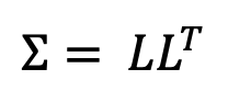
whereΣ represents the covariance matrix of asset returns. This transformation allows uncorrelated random shocks to be recombined into correlated outcomes that maintain the statistical properties observed in historical data or model assumptions.

Why this matters for financial advisers

For advisers constructing multi-asset portfolios, this technique provides a powerful framework to:

• Assess true diversification – understand how portfolios behave when correlations change in downturns.
• Model downside scenarios – estimate the probability and severity of large losses.
• Improve risk conversations – explain risks and outcomes to clients with data-driven clarity.
• Refine portfolio construction – test different asset allocations and see how risk and return distributions shift.

Implementation: Python vs Excel

While the theory may sound complex, applying Cholesky decomposition in practice is surprisingly simple – with the right tools.

In Python:

The numpy library can perform a Cholesky decomposition in just one line:

• L = np.linalg.cholesky(cov_matrix)

This allows advisers or analysts to integrate it directly into their simulation models, running thousands of portfolio trials efficiently.

In Excel:

• Excel does not have a built-in Cholesky function. To achieve the same result, one must use Visual Basic for Applications (VBA) – writing several lines of code to perform the decomposition and recombination. This is more time-consuming, harder to audit, and less scalable for larger datasets.

For advisory teams conducting frequent portfolio testing or building internal risk dashboards, Python’s simplicity, speed and repeatability make it the preferred choice.

Comparing the Results: Cholesky vs Non-Cholesky Simulation

The analysis is based on two representative assets with expected annual returns of 5 per cent and 7 per cent, and volatilities of 10 per cent and 15 per cent, respectively. A correlation of 0.6 is applied to reflect a moderate, realistic relationship between asset classes such as equities and property. This correlation defines the covariance matrix used in the Cholesky decomposition, ensuring that simulated return paths capture how assets typically move together under varying market conditions.

A parallel simulation assumes the assets are independent, maintaining identical return and volatility parameters but removing the correlation structure. This contrast isolates the impact of correlation on portfolio outcomes. Each model generates 100,000 Monte Carlo observations, with portfolio returns calculated using a 70/30 allocation.

The top panels show simulated asset returns.

• With Cholesky (top left): Returns display an elliptical pattern, indicating realistic co-movement between the two assets (ρ ≈ 0.6).
• Without Cholesky (top right): Returns scatter randomly, suggesting no correlation which is an unrealistic assumption that exaggerates diversification.

The bottom panels illustrate the resulting portfolio return distributions (70/30 weighting).

• With Cholesky (bottom left): The wider spread and thicker left tail capture real-world risk when assets move together in downturns.
• Without Cholesky (bottom right): The narrower, smoother shape underestimates volatility and downside potential.

Collectively, these plots underscore the critical role of correlation integrity in portfolio risk modelling. Incorporating Cholesky decomposition ensures that simulations reflect the genuine inter-dependence of asset returns, preserving the complex co-movements that occur across market cycles. This methodological precision produces a more faithful representation of portfolio dynamics, particularly under stress, when correlations typically converge and diversification benefits diminish.

Practical use cases

Cholesky-recomposited Monte Carlo simulation can enhance portfolio analysis in several ways:

• Stress Testing – Simulate severe downturns to see how portfolios might perform under simultaneous equity and bond sell-offs.
• Tail Risk Analysis – Estimate Value-at-Risk (VaR) and Conditional VaR, helping advisers understand extreme loss probabilities.
• Scenario Planning – Examine how portfolio outcomes might change if volatility doubles or correlations spike.
• Diversification Validation – Assess whether current diversification truly holds up when markets become turbulent.

This approach turns traditional “average-based” thinking into a probability-based understanding of risk, enabling more confident, data-driven client conversations.

Cholesky-recomposited Monte Carlo simulation provides a powerful, modern framework for financial advisers to analyse portfolio risk. It goes beyond static performance charts, offering a dynamic, correlation-sensitive view of portfolio behaviour.

While Excel remains useful for simple analysis, Python’s ability to run complex mathematical operations – like Cholesky decomposition – in a single line makes it a superior choice for robust portfolio simulation.

By embracing these quantitative tools, advisers can move from describing the past to anticipating the future, empowering clients with greater transparency and confidence in their investment strategy.

Ye Peng